Bias-Variance-Noise From First Principles
Imagine you are studying a real world phenomenon. You notice it takes some input and gives an output. You take an infinite number of observations. Finally you notice that for the same input, the system gives you slightly different outputs each time.
You think better equipment might help get rid of the error, and decide to spend millions. The equipment arrives, you repeat the experiments, and the error decreases but not by much.
In fact you can keep buying more accurate equipment, but the error never goes away. This is an inherent, irreducible noise of the system.
You come to the conclusion that there is a true function underneath, unobservable because of the noise.
Mathematically
where y is the observed output, f is the true unknown function, x is the input, and ε is irreducible noise with mean 0 and variance σ².
Since we don't know the true function f, we train a model f_hat on a dataset d sampled from the population D.
Now imagine training infinitely many such models, each time on a different dataset randomly sampled from D.
Each model is slightly different, because the sample dataset d changed; function remained the same.
We define f_bar as the average prediction across all these models.
f_bar is just a number - the randomness over datasets has been averaged out.
Our goal now is to decompose equation (I) so that the irreducible noise separates out cleanly from the model's own errors.
Step 1. Insert ±f_bar into the error.
The cross term has two factors. They are independent because y does not depend on which dataset d was drawn, y comes from nature, f_hat comes from training. Since they are independent, the expectation of their product is the product of their expectations.
From (II), E[f_bar - f_hat] = f_bar - f_bar = 0. The signed deviations of f_hat around its own mean always cancel (definition) So the cross term vanishes.
Step 2. The first term still mixes noise and bias together. We can see this because y still contains ε. So we need to split again. Insert ±f(x).
Since y = f(x) + ε and E[ε] = 0, we have E[y - f] = 0, so the cross term vanishes again.
And E[(y - f)²] = E[ε²] = σ² (variance of the noise).
So the first term becomes -
Step 3. Substituting back, and noting that f_bar = E[f_hat] from (II).
What each term means...
Bias² = (f - E[f_hat])²
The gap between the true function and the average model. If your model family is too simple, say, a straight line trying to fit a curve - it will be systematically wrong no matter how much data you give it. More data does not fix bias. Only a more expressive model does.
Variance = E[(f_hat - E[f_hat])²]
How much individual models scatter around their average. A very flexible model trained on two different datasets gives two wildly different answers - high variance. It is sensitive to the specific sample it saw, memorising noise rather than learning signal. Fixed with more data, simpler model, regularization (more on this in another blog), & ensemble.
Noise = σ²
The irreducible floor. Even a perfect model that knew f(x) exactly would still incur this error, because the observations themselves are noisy. No amount of data, model capacity, or clever training eliminates it.
These three terms are completely independent and sum exactly; no approximation was made.
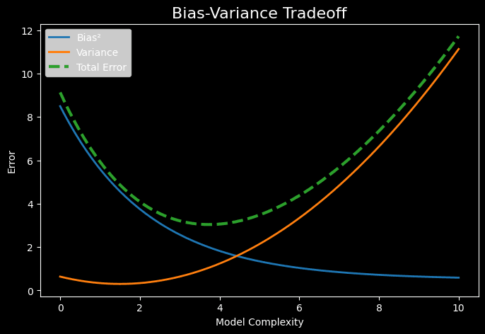
The Trade-off
The practical consequence is a tug-of-war: the same knob that reduces bias (more model complexity) increases variance, and vice versa. A too-simple model underfits - high bias, low variance. A too-complex model overfits - low bias, high variance. The goal is the complexity level where their sum is minimized.
In modern overparameterized models there is a secondary effect - double descent - where this simple U-shaped tradeoff breaks down. But that is a story for another time.
Practicality
Theoretically this decomposition is clean, but in practice we never have access to f(x) or σ². We can't compute bias or variance directly. Instead we use proxies that estimate total expected error.
| Method | What it estimates | What it says |
|---|---|---|
| Train/test split | Total expected error | Fast but noisy |
| k‑fold cross‑validation | Total expected error | Lower‑variance estimate, good for comparing models |
| Learning curves | Relative bias vs variance | Which problem dominates |
| Noise floor | σ² (irreducible error) | Whether further improvement is possible |
Training curves give a real‑time diagnosis of bias vs variance. The two key signals are - absolute train loss (bias indicator) and gap between train and validation (variance indicator).
- Training loss high, validation loss high, & close together -> high bias (underfitting)
- Training loss low, validation loss high & widening -> high variance (overfitting)
- Both losses low with a small stable gap -> good generalization (near noise floor)
- Both losses still decreasing -> undertraining
Fighting the imbalance
Almost every fix trades one for the other. Reducing bias usually increases variance, and vice versa. The art is in minimizing the total error.
High bias
The model is systematically wrong, it cannot represent the underlying function even with infinite data. The fix is more expressive/flexible model or better information.
- Increase model complexity -> deeper networks, more trees, higher‑degree polynomials
- Reduce regularization -> lower L2/L1 penalties, reduce dropout
- Add richer features -> interaction terms, domain‑specific features, embeddings
- Improve data quality -> cleaner labels, higher‑resolution inputs
- Train longer -> underfitting often comes from incomplete optimization
High variance
The model fits the training set too closely and fails to generalize. The fix is to constrain it. All regularization trades a small increase in bias for a larger decrease in variance.
- L1 regularization -> drives weights to zero, performing implicit feature selection
- L2 regularization -> penalizes large weights, producing smoother predictions
- Dropout -> forces redundancy, approximating an ensemble
- Early stopping -> prevents memorizing noise
- Data augmentation -> more effective samples, reducing sensitivity
Side note - bias is a loaded term
The word bias shows up in several different contexts in machine learning, and they don’t all refer to the same thing. Bias-variance bias is the statistical notion (discussed in depth above). Neuron bias (b in wx + b) is a learnable offset that shifts an activation function, it inherited the name from statistics in the 1950s and it stuck. Dataset bias refers to training data that fails to represent the true population (loosely related to b-v). & algorithmic or societal bias describes unfair or discriminatory patterns a model may learn from data.
Well, I really enjoyed writing this piece and hope you enjoyed reading it just as much; next, I’ll be exploring the geometric intuition behind L1 & L2 regularization, circle back to how they shape variance. Stay tuned! :)